Introduction
Floods are among the most common and dangerous natural disasters worldwide. A deeper understanding of the flood hazard phenomenon and its potential consequences for society is considered a fundamental criterion for developing effective flood management policies, risk reduction projects, and other flood-related strategies (Amrei & Britta, 2022). Over time, the need for protection against floods and the ability to control them led to a shift in perspective on flood control and management. Modern concepts of flood risk management began to emerge in the early 20th century. With the development of research and the increase in losses caused by floods, a need was felt for a new approach that applies the concept of risk in decision-making, not theoretically, but practically (Alexander & Mees, 2016). Flood risk is the result of the interplay between flood hazard (probability and severity) and the vulnerability of people and their property. Both hazard and vulnerability depend on the type of flood and its determining processes (Yin et al., 2021). Flood risk studies indicate that the flood hazard maps, along with economic assessments, are used as planning and decision-making support tools (Dalledonne et al., 2019). Therefore, it is essential that methods and tools for examining adverse flood outcomes are presented in a comprehensive, coherent, and inclusive manner to enable competent authorities and experts to make decisions by identifying priority solutions through a balance between economic/social/ environmental functions and social conflicts.
Flood risk assessment includes three components: Hazard, vulnerability, and exposure analysis (Liu & Merwade, 2014). Flood hazard mapping is usually done using hydrological and hydraulic models and field surveys. The process of preparing such maps, which ranges from data collection to modeling, is accompanied by a series of uncertainties. Conventional hydraulic-hydrodynamic modeling methods can lead to inaccurate results due to neglect of sources of uncertainty (Alfonso et al., 2016). Despite the development of many hydraulic models, the lack of understanding of flood processes and the spatial and temporal variations of key model inputs, as well as variables such as topography and surface roughness, hinders the better prediction of flood risk. Measuring and reducing uncertainty in flood modeling is an important issue for improving the accuracy of flood forecasting (Teng et al., 2017). 
The precision of the models used in flood risk simulation has a significant impact on the efficiency of flood risk management (Merwade et al., 2008). Of course, uncertainty cannot be avoided in the use of flood analysis models, because these models often capture ideals of reality only and the value of model inputs cannot be measured with absolute resolution (Yeou-Koung & Chi-Leung, 2016). Various sources of uncertainty in hydrological and hydraulic modeling include: Natural (intrinsic) uncertainty; uncertainties related to the model structure, parameters and input data; and operational uncertainties (Teng et al., 2017; Koo et al., 2020). Natural uncertainties are related to natural random processes such as precipitation, turbulent river flow, and sediment transport; model structure uncertainties stem from the mathematical structure of the processes and the inability of model equations to accurately describe real systems; parameter uncertainties are related to imprecision in determining parameter values, as well as data and information uncertainties resulting from measurement errors, data heterogeneity, and information deficiencies; operational uncertainties are related to model construction and development, as well as human factors (Dysarz et al., 2019). In this regard, preparing a digital elevation model (DEM) with appropriate precision as large-scale topographic data is considered one of the most sensitive factors and inputs of hydrodynamic models.
Several studies have investigated the impact of the resolution of DEMs on the simulation of hydrological processes and flood risk zoning. Among these studies, we can mention the study by Kavian and Mohammadi (2019) on the effect of spatial precision of DEMs on simulation of discharge and total nitrate in the Talar watershed, Mazandaran province, Iran, using the SWAT model and three different DEMs (ASTER with a resolution of 30 meters, SRTM with a resolution of 90 meters, and GTOPO30 with a resolution of 1000 meters). Their results showed that the ASTER model had higher accuracy and provided the best simulation results. As the spatial precision decreased, the overestimation or underestimation error rate also increased. In a study by Parizi and Hosseini 2023, the TanDEM-X model with a resolution of 12 meters was used to simulate the hydraulic characteristics of floods in the Atrak River basin. In their study, which was conducted with the HEC-RAS 2D model, the results showed that TanDEM-X was able to model the flood extent with an accuracy of over 85%. Comparison with the ASTER and SRTM models showed that TanDEM-X was significantly more accurate and had a high ability to display topographic details. In a study by Fereshtehpour et al. (2024), the effect of DEM type and resolution on flood prediction using one-dimensional convolutional neural networks was investigated. They used elevation data with accuracies of 15 and 30 m in the city of Carlisle, England, and found that DTM-type DEMs with a precision of 30 m performed better in predicting flood depths compared to DSM-type DEMs. Increasing the precision to 15 m increased the root mean square estimation by 50%, indicating the sensitivity of the model to the precision of the DEM. Muthusamy et al. (2021) investigated the impact of DEM resolution on urban flood modeling. They showed that reducing the resolution of DEM from 1 m to 50 m resulted in a 30% increase in flood extent and a 150% increase in flow depth, highlighting the importance of using high-accuracy DEMs in urban flood modeling. In a study in southern Niger, Muench et al. (2022) evaluated the accuracy of global DEMs such as SRTM, ASTER, ALOS, and MERIT in flood modeling. They found that the ALOS-type DEM had the best similarity to LiDAR data, and that in floods less than 3 m deep, higher-accuracy DEMs showed a greater similarity in estimated flood extent to measured values. 
The review of the literature showed that the effect of the resolution of DEMs on the efficiency of the HEC-RAS hydraulic model in simulating flood hazard zones has received less attention, especially in Iran. Therefore, this study aims to evaluate the impact of the resolution of DEMs on the efficiency of the HEC-RAS model in mapping flood hazards in a 3-kilometer-long area of the river downstream of Khorramabad City, Iran.

Materials and Methods

Study area
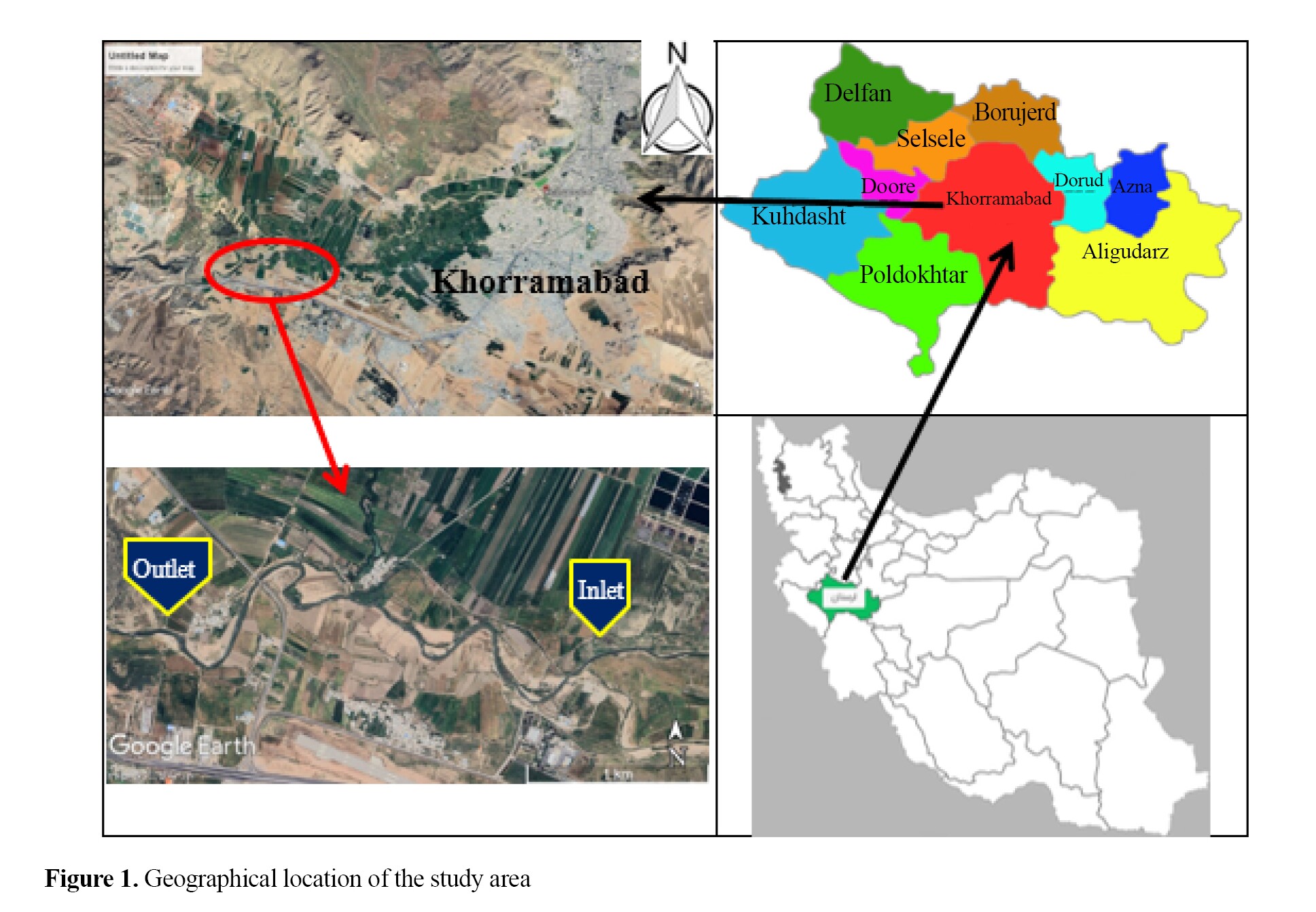
The study area is located 3 km downstream of Khorramabad City, Lorestan province, in an area called Cham-Anjir, which is actually the outlet of the Khorramabad river watershed. The study area is located between geographical coordinates of X: 247128.7, Y: 3704013.16 (inlet of the area) and X: 245084.7, Y: 3704099 (outlet of the area), as shown in Figure 1. The watershed of this river is a sub-watershed of the Kashkan River. The Khorramabad River is formed by the confluence of the two headwaters of the Karganeh and Robat in Khorramabad and joins the Kashkan River in Doab town, 40 km from Khorramabad. The Cham-Anjir hydrometric station is located at the outlet of the study area.

Hydrodynamic model
Two-dimensional (2D) hydrodynamic models are the most useful models for flood mapping and flood risk assessment (Roberts et al., 2015). In this study, the 2D HEC-RAS 5.0.1 model, developed in February 2016, was used. In addition to one-dimensional modeling of steady, unsteady, and quasi-steady flows, as well as intersectional and lateral structures, this model also has the capability for 2D flow modeling, especially in floodplains. One-dimensional models are efficient and capable of reproducing processes within channels, but problems begin when flood overflows the channel banks and enters the floodplain (Pinos & Timbe, 2019; Costabile et al., 2020). This model is one of the most common flood modeling software in hydrodynamic simulation, developed by the US Army Engineer Hydrologic Engineering Center (HEC). It can connect to online maps such as Google Earth. The HEC-RAS model uses the 2D Saint-Venant equations (with optional momentum additions for turbulence and Coriolis effects) or 2D diffusion wave (DW) equations to simulate the flow. In general, 2D DW equations enable the model to run faster and achieve much greater stability. In the 2D HEC-RAS model, it is possible to choose one of these two equations based on the available data and the type of project (Brunner, 2016).

Topographic map and measurement of water flow variables
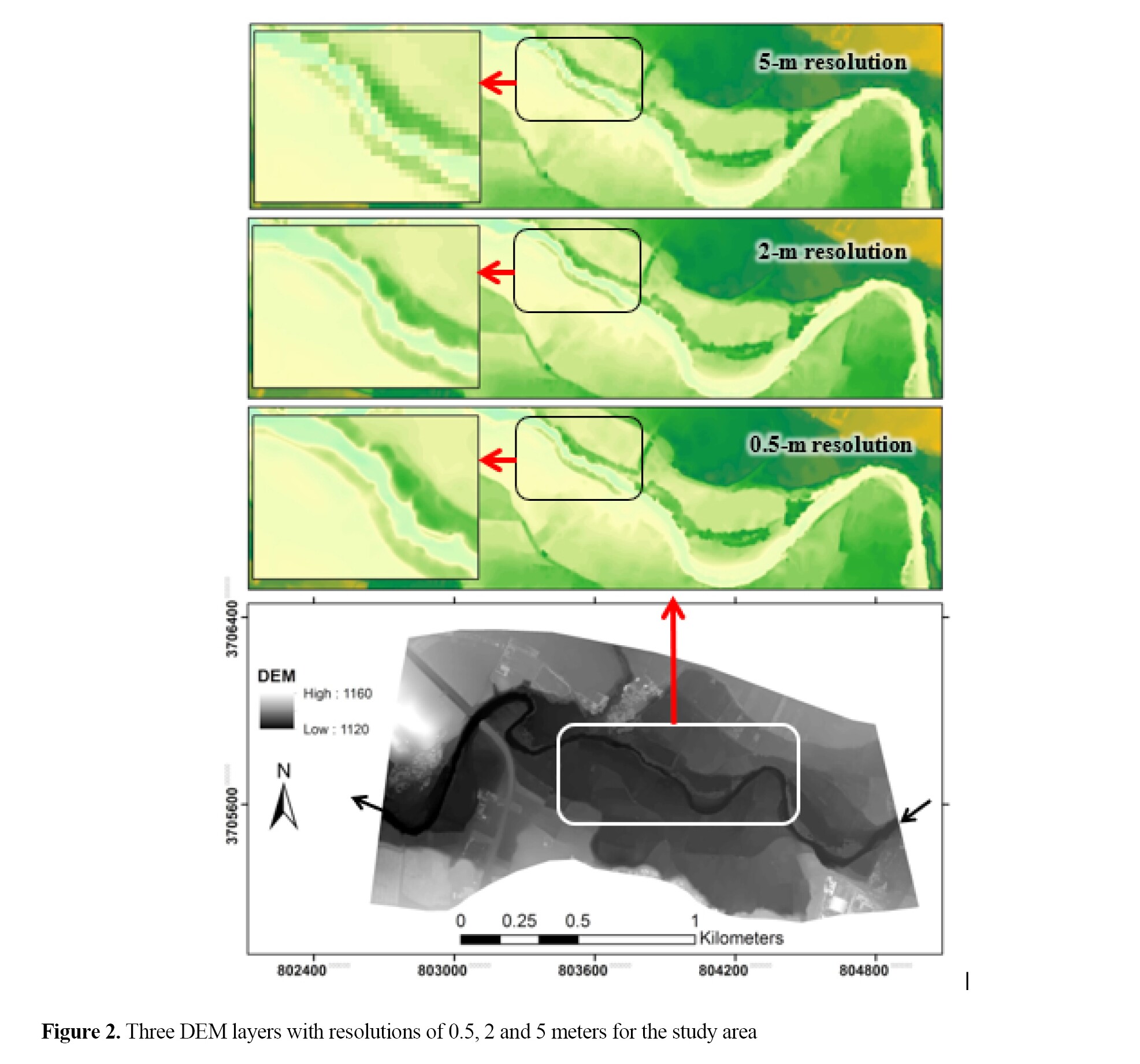
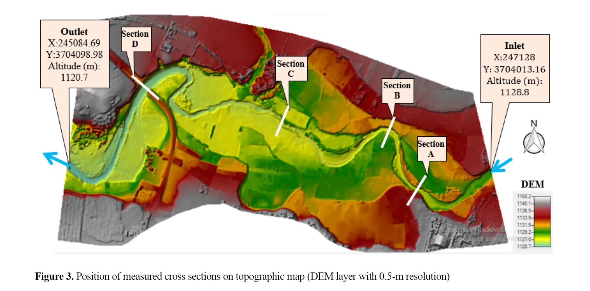
To determine the effect of the resolution of the DEMs on the HEC-RAS model results, three DEM layers were prepared with resolutions of 0.5, 2, and 5 meters. The layer with 0.5-m resolution was generated from 2024 Worldview stereo imagery developed by DigitalGlobe Inc; validated using several control points with a field mapping camera (Fiureg 2 and 3). and the layers with 2- and 5-m resolutions were generated from 2023 drone maps, prepared from the Regional Water Company in Lorestan Province and verified using a number of control points with a field mapping camera (Fiureg 3). Large-scale topographic maps were converted to .hdf format for loading into HEC-RAS software. After entering the geometric data into the software and determining the boundaries, the desired area was gridded using algebraic and computational methods. The optimal grid dimensions were selected based on the required accuracy and the time allocated for the calculations (Fiureg 4). 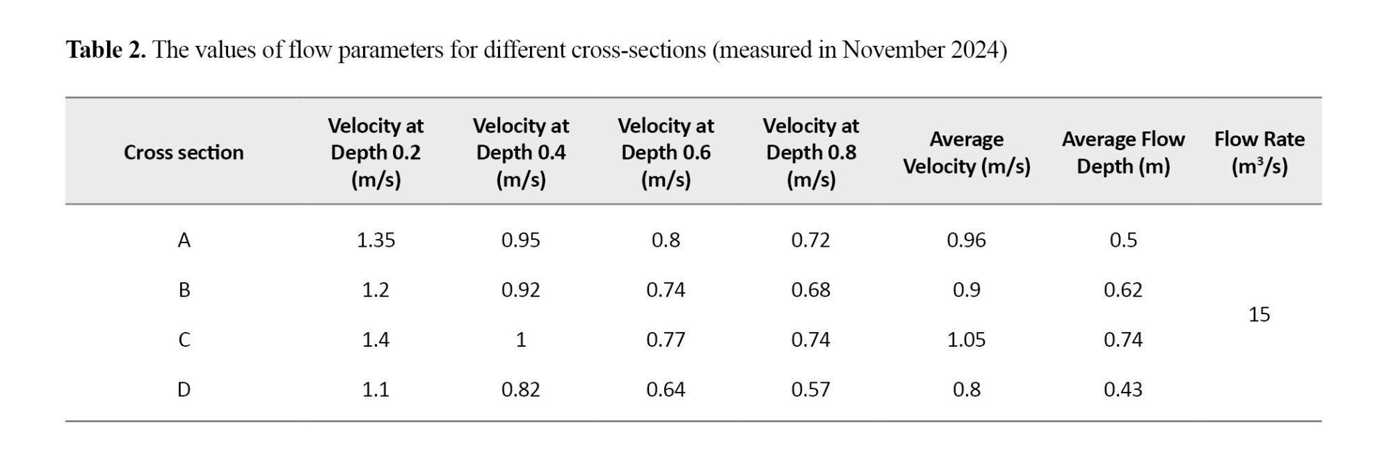To evaluate the calibration and accuracy of the model results, flow parameters (velocity, depth, and spread width) were measured in four of the mapped cross sections, with the greatest emphasis on consecutive river bends to examine the effects of secondary flows and centrifugal forces on flow variables. A Moulinet speedometer and computational mesh were used to measure the flow velocity and depth (Fiuregs 4 and 5). 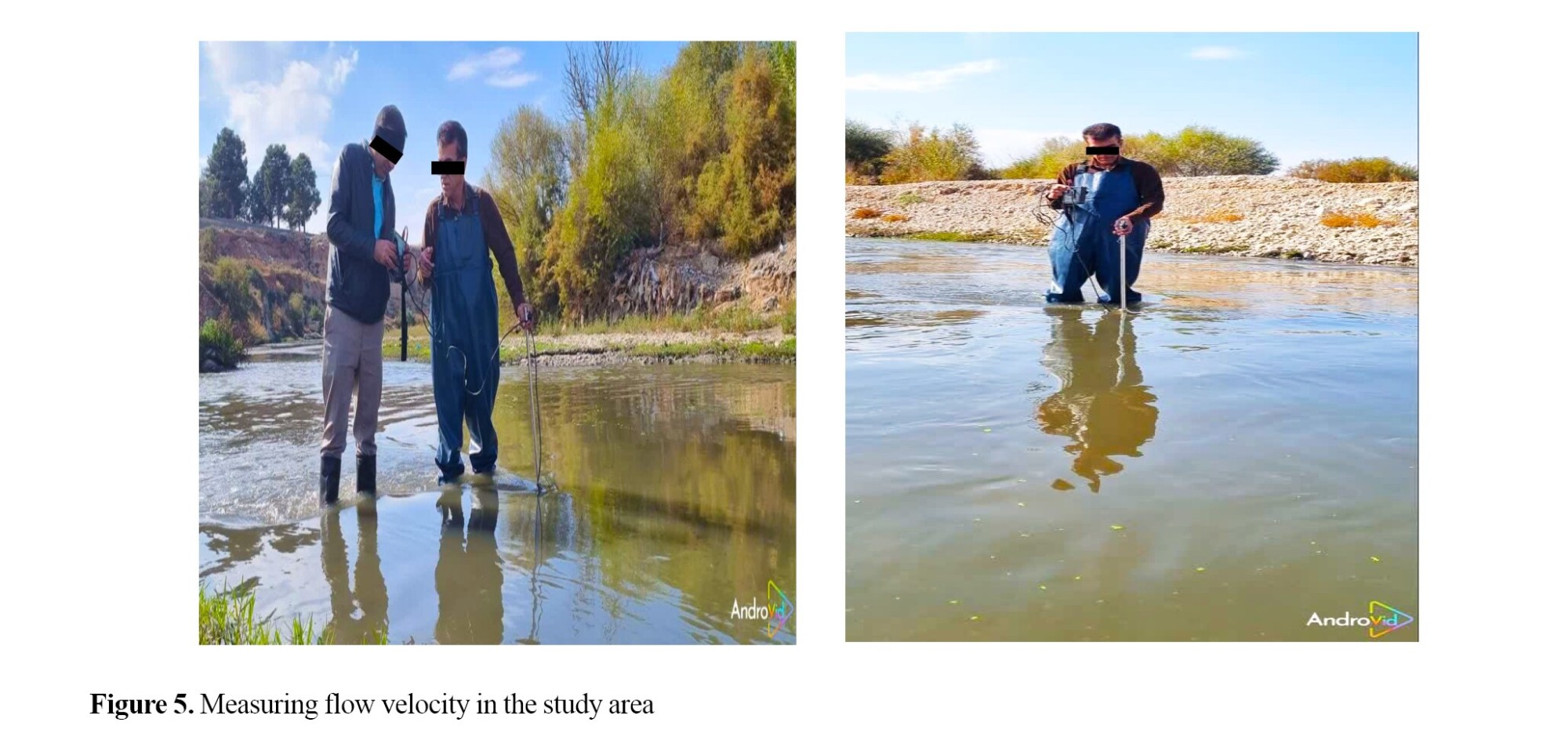The flow velocity was measured using a speedometer at depths of 0.2, 0.4, 0.6, and 0.8 meters below the water surface (Alizadeh, 2010). Since in flood flows, the velocity varies at different points of the river and at different water depths and is accompanied by turbulence, the average flow velocity in each cross-section (considering the width of each section) was measured at 6-10 points with equal distances from the water depth.
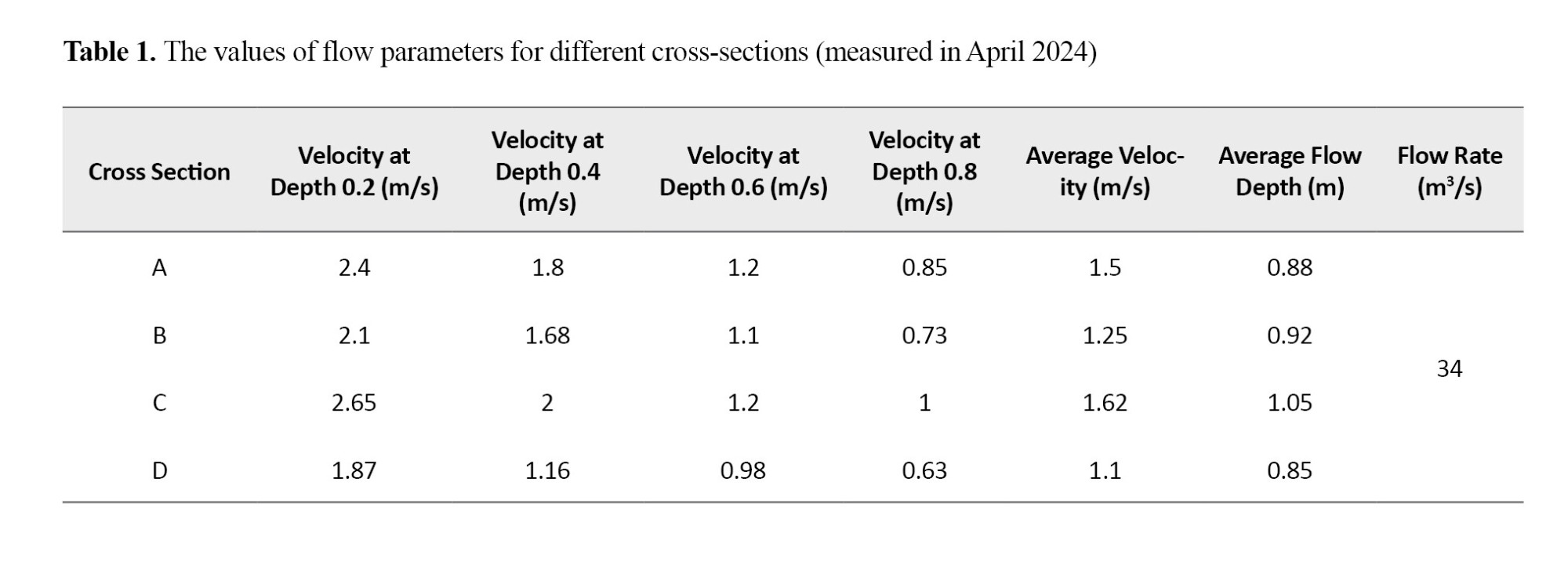
Tables 1 and 2 show the values of flow velocity, flow rate, and flow depth for different cross sections measured in April and November 2024, respectively. The criteria for field measurement of depth and width at the flood flow (1000 m3/s) were based on the results of the overflow water and flood extent determined by the Regional Water Company in Lorestan Province. In other words, based on the flood extent and the height difference between the overflow line and the elevation level at different points of a cross-section, the flood flow depth at different points of a cross-section was obtained and used as a criterion for model calibration and validation.

Determining the roughness coefficients
Understanding the factors affecting Manning’s roughness coefficient is a good way to estimate this coefficient more accurately. These factors include: Roughness of the riverbed or the type and grain size of riverbed materials, roughness degree of the riverbed surface, presence of obstructions in the channel and changes in its cross sections, type and density of vegetation cover, shape and size of the channel, and even hydraulic conditions such as flow depth and discharge which, in addition to affecting the longitudinal loss in the flow path, somehow have a role in losses due to flow deformation (local losses). Among the methods available for estimating Manning’s roughness coefficient, Cowen’s method includes the role of all the aforementioned factors in its calculations (Arcement & Schneider, 1989). Manning’s roughness coefficient (n) by this method is defined as (Equation 1):
1. n=(nb+n1+n2+n3+n4 )×m
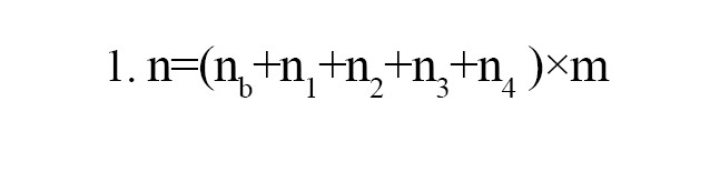
Where, nb: Base value of roughness coefficient according to the bed material and grain size of the river bed materials in the case of a smooth and straight channel; n1: value of roughness coefficient related to the surface irregularities; n2: value of roughness coefficient for variations in the channel cross section; n3: Value of roughness coefficient for obstructions; n4: Value of roughness coefficient for vegetation; and m: Value of roughness coefficient for meandering of the channel. The value and method of selecting these coefficients are included in the tables and instructions in the open-channel hydraulics books (Trinh et al., 2021) and also in the study by Arcement and Schneider (1989).
To determine the roughness coefficient n, the study area was first homogenized based on field visits to the river and observations of changes in effective parameters, considering morphological status and land uses. Then, the roughness coefficient values were determined based on the photographs and descriptions contained in Chow’s open-channel hydraulics book and other sources, such as the USGS reference. The values ​​were determined for different cross sections according to all effective parameters.

Determining boundary conditions
Boundary conditions include the inflow and outflow conditions of the study area. Considering the steady or unsteady state of the flow and the available information (flow hydrograph, water surface level, and flow rate-water surface level relations), they were considered as flow boundary conditions. In this study, the boundary conditions for simulating unsteady river flow were determined based on observational statistics from the Cham-Anjir hydrometric station for three events: The flood event in April 2019, the water flow discharge on 04/12/2024, and the water flow discharge on 11/15/2024.

Model calibration
To simulate river flow using the 2D HEC-RAS in the study area, ​​the objective function needs to be optimized by adjusting some parameters of the roughness coefficient (Trinh et al., 2021). Also, the lack of access to recorded data of large historical floods, such as the flood event that occurred in April 2019 in the study area, poses a serious problem for model calibration. Therefore, for this event, a simulation operation was performed based on data on the overflow water, flood depth, and the upper flood level (Pinos & Timbe, 2019). The model was calibrated by optimizing the Manning’s roughness coefficient values ​​for the flood event in April 2019 (daily peak flow rate =1000 m3/s) based on the overflow level and flood spread width, and also for the water flow hydrograph in April and November 2024 based on field measurements of flow variables, including depth and velocity, at four cross sections of the study area.

Sensitivity analysis of the HEC-RAS model
Changes in the resolution of the DEM lead to changes in the geometry of the river channel and, consequently, to changes in the pattern of water flow variables. One of the most important sources of uncertainty in the results of hydraulic models is related to related to the model parameters. Therefore, in this study, an attempt was made to evaluate the sensitivity of the 2D HEC-RAS model to the resolution of DEMs. In this regard, the simulation results, including the depth and velocity of water flow, based on the three DEM layers with resolutions of 0.5, 2, and 3 meters, were compared with the measured values in four cross sections of the study area for the aforementioned flow rates. The analyses were performed along with measuring the root mean square error (R.M.S.E) and mean absolute percentage error (M.A.P.E) as follows (Equations 2, 3):
2. 
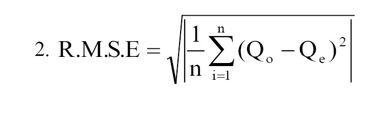
Where Qo is an observed value and Qe is the calculated value of the model
3. 
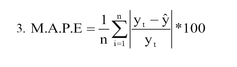
Where yt is an observed value and  is the calculated value of the model.

Results

Calibration and sensitivity analysis of the 2D HEC-RAS model
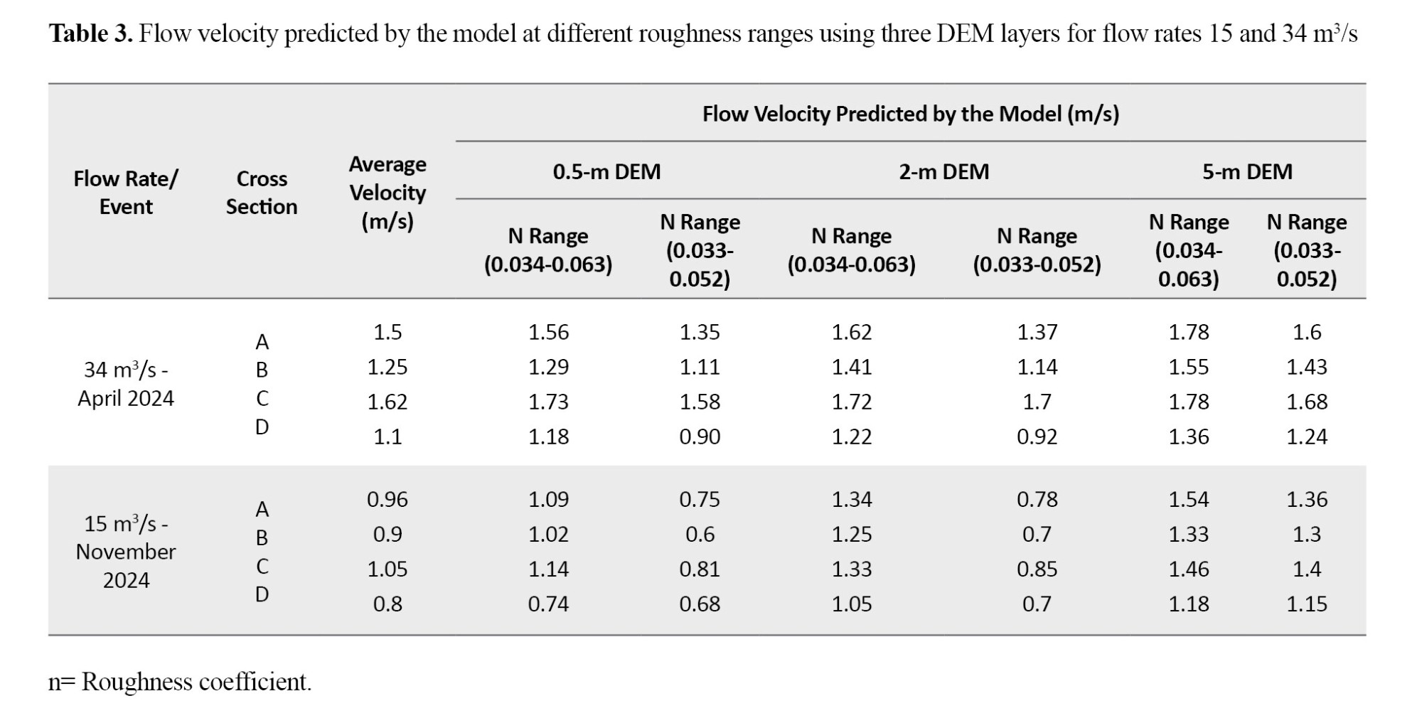
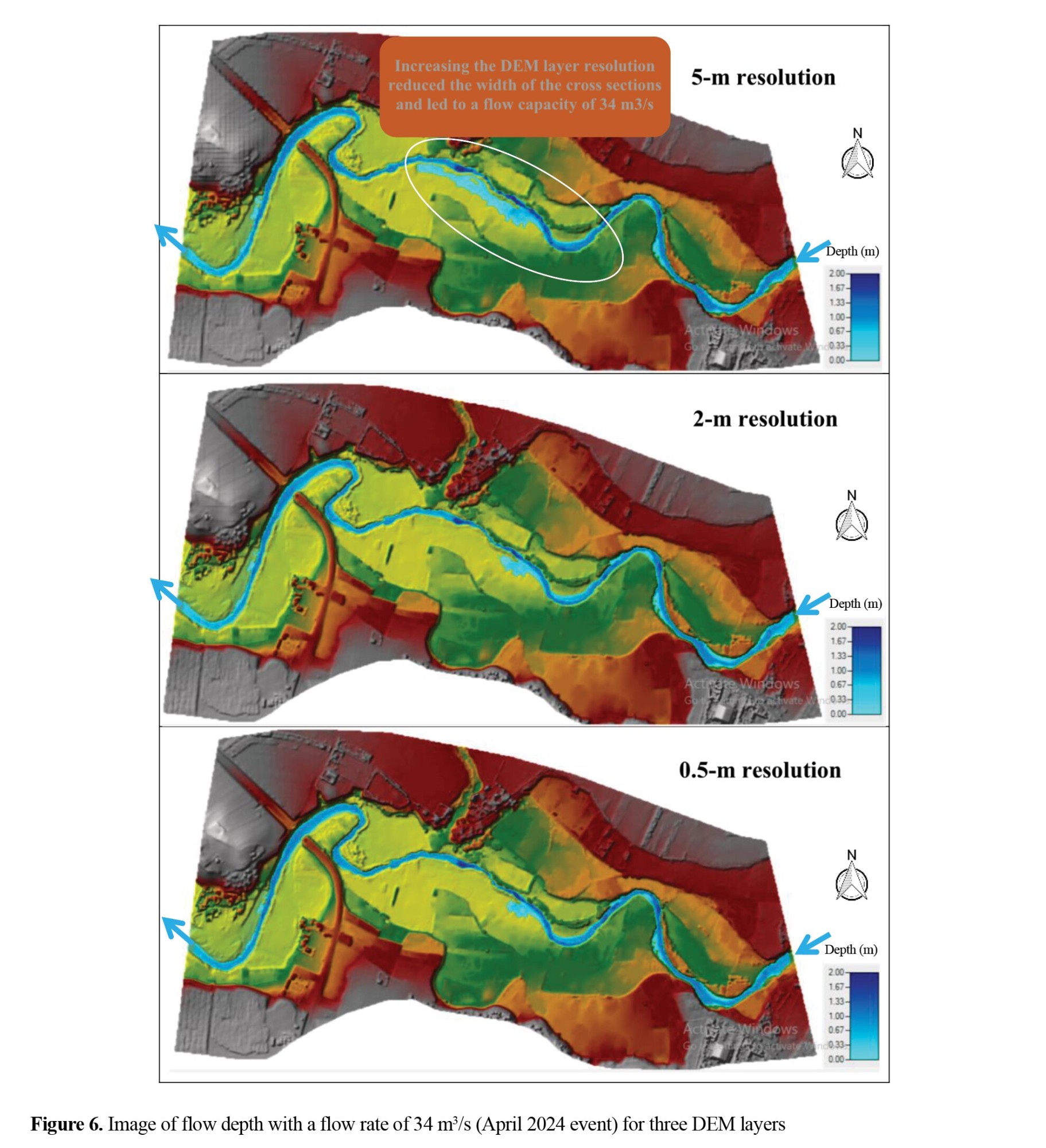
The results of the velocity, depth, and width of the flow extent for three DEM layers compared to the results measured at different cross sections (A, B, C, D) are presented in Tables 3 and 4 and Figures 6 and 7. As shown in Table 3 and Figure 6, for the flow rates measured in April and November 2024, the predicted values closest ​​to the observational values (velocity, depth, and spread width) of the water flow in the four cross sections were related to the DEM layer with 0.5-m resolution followed by the layers with 2- and 5-m resolutions, and the roughness coefficient was in the range of 0.033-0.063. At these flow rates, the difference in the estimated values ​​of water flow variables was significant using the 5-m DEM layer compared to when the layers with 0.5 and 2 meters of resolution were used. This is due to the variations in the geometry of the full cross-section channel with the change in the dimensions of the DEM layer. In particular, this change affected the full cross-section channel width; as the dimensions of the DEM layer increased, the full cross-section channel width decreased. Therefore, these changes in the channel geometry have led to changes in the depth and velocity of water flow in the full cross-section channel.
As shown in Table 4 and Figure 7, for the April 2019 event with a flow rate of 1000 m3/s, similar to the flow rates measured in April and November 2024, the predicted values closest ​​to the observational values (depth and spread width) of the water flow in the four cross sections were related to the DEM layer with 0.5-m resolution followed by the layers with 2- and 5-m resolutions, and the roughness coefficient was in the range of 0.033-0.063. 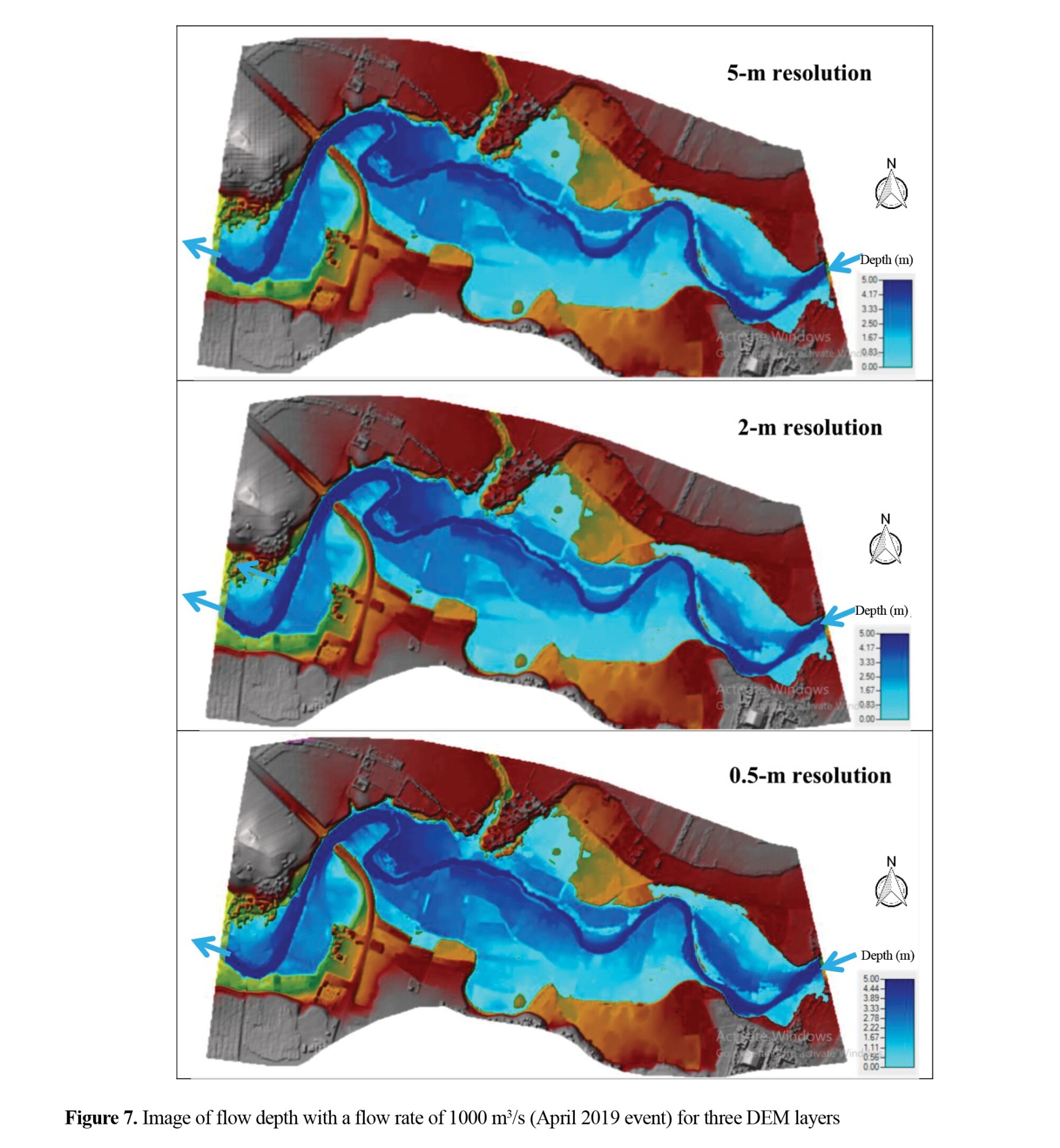However, at the flow rate of 1000 m3/s (for the April 2019 event), the difference in flood flow variables (flow depth and velocity) among the three DEM layers was not significant. Therefore, when the water flow rate increases to the point where it moves out of the channel and enters the floodplain, and the flood extent width becomes several times more than the width of the water surface in the full cross-section channel, the effect of increasing the DEM layer resolution from 2 to 5 meters on the flood flow depth and velocity is not significant.
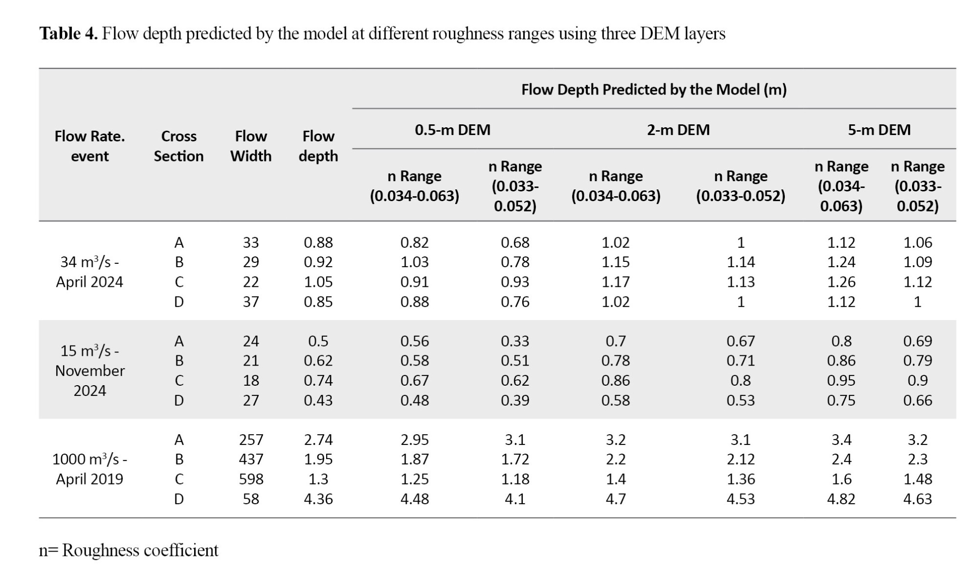
For a flow rate of 34 m3/s, the maximum flow depth caused by the narrowing of the channel at several sections and the centrifugal force in the concave curve was 2 meters. Due to the high curvature in the arches of the study area, maximum flow changes (increase in velocity) occur in the second half of the arch (Figure 6). On the other hand, as shown in Figure 7, for a flow rate of 1000 m3/s (April 2019 event), the maximum flow depth at the bridge location (section D) was 5 meters. The entire territory of the study area does not have the capacity to pass this flood; therefore, the flood overflows 95% of the banks and spreads to the flood plain. The largest flood spread width of about 600 meters occurred at section C, and the smallest flood spread, due to the presence of a transverse obstruction, was at the bridge location (section D). Also, for this event (April 2019), given that the flood spread widely to the banks, the water velocity was affected by flow turbulence, trend, topography, and obstructions in the floodplain. For these conditions, the flow velocity in the study area lacks a stable pattern; with changes in the flow rate, the flow velocity pattern changes throughout the study area. For the April 2019 event, the highest water flow velocity due to the transverse obstructions was seen at the bridge location (section D).
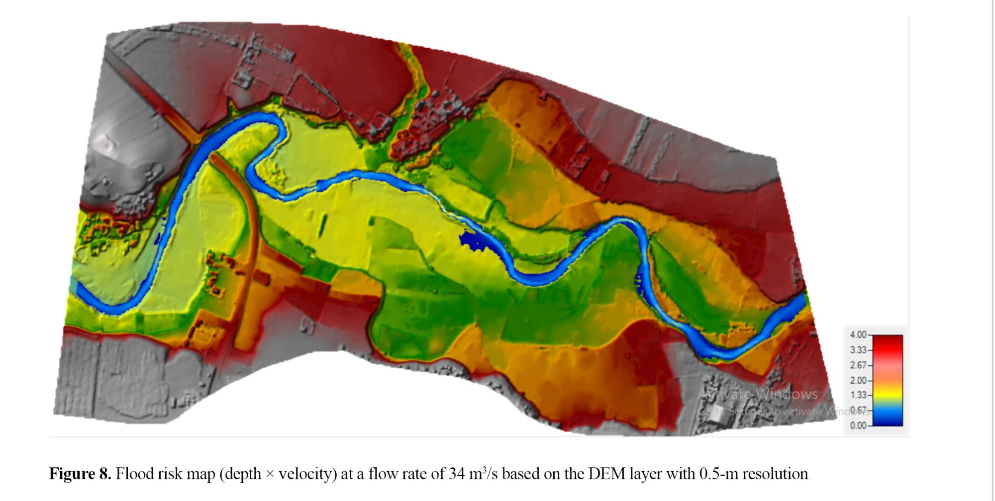
As shown in Figures 8 and 9, for a flow rate of 34 m3/s and the 0.5-m DEM layer, given that the study area had the capacity to pass this flow, the quantitative values ​​of the flood hazard zone were less than the threshold limit. Therefore, the flood risk in these conditions is at a normal level. For the April 2019 event with a flow rate of 1000 m3/s, generally, the highest numerical flood risk level was in the full cross-section channel of the study area, but specifically, the highest flood risk was in the third arch/bridge location (section D). On average, the transverse extent of the flood, with a value greater than 10, was approximately 160 meters. In the arches of the studied area, the maximum flood hazard occurs on the outer side of the arches.
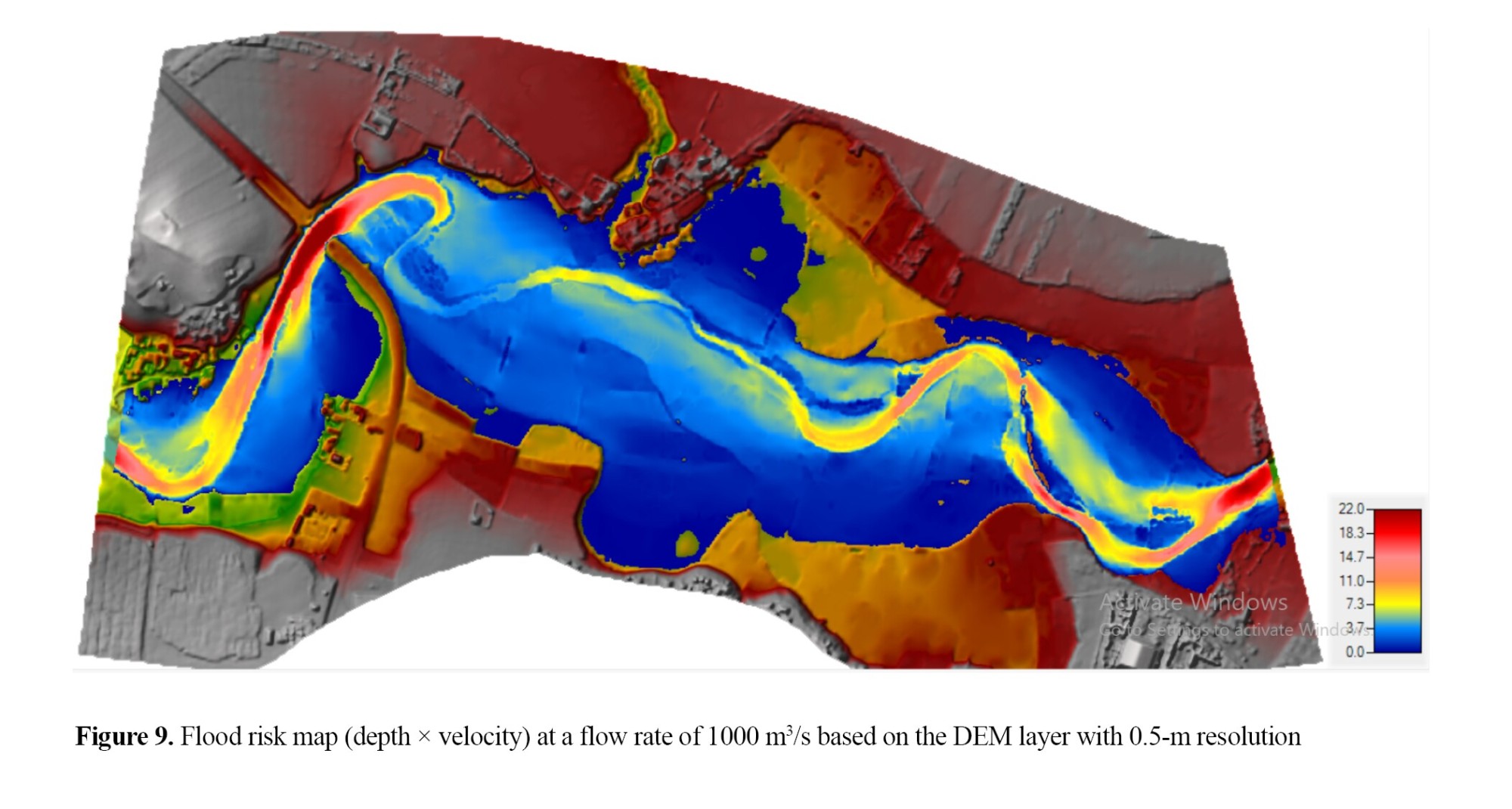
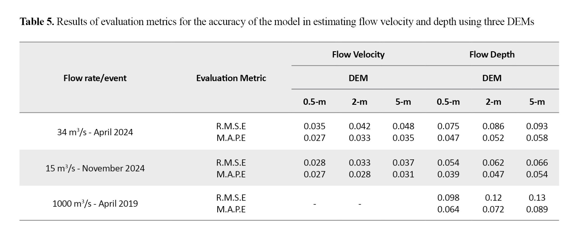
Table 6 shows the accuracy of the 2D HEC-RAS model in estimating the parameters of flow velocity and depth using three DEMs with resolutions of 0.5, 2, and 5 meters and based on the R.M.S.E. and M.A.P.E. evaluation metrics. As can be seen, for the three events studied, the lowest evaluation metrics for predicted values (velocity and depth) ​​compared to observational values were related to the DEM with resolutions of 0.5 and 2 meters.

Discussion
The findings of this study, which demonstrated the superiority of DEM with 0.5-m resolution in flood risk simulation, are consistent with the results of Muthusamy et al. (2021) and Fereshtehpour et al. (2024), who showed that high-resolution DEMs (0.5-1 m) significantly reduce flood risk zoning errors. The study by Parizi and Hosseini (2023) also revealed that the TanDEM-X model with a resolution of 12 meters had a significant error in estimating flood depth compared to local DEMs with a resolution of 1 meter, which confirms the importance of the spatial accuracy of DEMs. This study’s recommendation for the use of high-resolution DEMs in flood management is in line with the recommendations of Alfonso et al. (2016) and Alexander and Mees (2016), who emphasized the role of accurate data in reducing flood risk.

Conclusion
One of the most important sources of uncertainty in the results of hydraulic models is the uncertainty related to the model parameters. On the other hand, the most sensitive stage in this field is the preparation of a DEM with appropriate precision and resolution. Therefore, in this study, by preparing the maps of flow depth, flow velocity, and flood risk in 3 km downstream of Khorramabad City, an attempt was made to evaluate the sensitivity of the 2D HEC-RAS model to the precision of DEMs with resolutions of 0.5, 2, and 5 meters. The results of this research show that the resolution of DEMs plays a key role in improving the efficiency of the HEC-RAS model for simulating the flood hazard zone. By using a DEM with 0.5-m resolution, we obtained simulation results that were closer to real (observational) data compared to the other two DEMS with lower resolutions (2 and 5 meters). These findings emphasize that high accuracy of elevation data is an effective factor in reducing the uncertainty of flood predictions.
The analyses showed that the geometric changes caused by the different resolutions of DEMs had a major impact on the flow depth, flow velocity, and flow spread width. When the water flow rate increases to the point where the water overflows the channel, the impact of DEM resolution on flood predictions is significantly reduced. This is important because in flood conditions, channel geometry and topography changes can lead to a decrease in the accuracy of predictions. For a flow rate of 1000 m3/s, given that the flood spreads widely to the banks, the water velocity pattern is affected by flow turbulence, flow direction, topography, and obstructions in the channel. For these conditions, the water flow velocity in the study area lacks a stable pattern, and with changes in the flow rate, the flow velocity pattern changes throughout the study area.
The results of the model sensitivity analysis showed that the 2D HEC-RAS model had high sensitivity to the equations used. The model’s performance in simulating the measured flow in April and November 2024, using the DW equations, was much better. In contrast, for the April 2019 flood event, the use of dynamic wave equations provided better results. Among the various hydraulic properties, the water surface level showed the least sensitivity to computational equations.
The results of this study can help in the optimal planning and management of water resources and reduce the damages caused by floods. Policymakers and water resources managers in Iran should pay special attention to the importance of DEM resolution in decision-making related to flood risk management so that they can develop effective programs to reduce damages and improve the resilience of communities against floods.

Ethical Considerations

Compliance with ethical guidelines
All ethical principles were observed in this study. Since there were no experiments on human or animal samples, the need for ethical code was waived.

Funding
This research did not receive any specific grant from funding agencies in the public, commercial, or not-for profit sectors.

Authors' contributions
Conceptualization, methodology and, initial draft preparation: Iraj Vayskarami and Ali Haghizadeh; Software, visualization, review and editing: Iraj Vayskarami, Ali Haghizadeh, and Aboalhasan Fathabadi; Supervision: Ali Haghizadeh; Final approval: All authors.

Conflicts of interest
The authors declared no conflict of interest.

References

Alexander, M., Priest, S., & Mees, H. J. (2016). A framework for evaluating flood risk governance. Environmental Science & Policy, 64(1), 38-47. [DOI:10.1016/j.envsci.2016.06.004]
Alfonso, L., Mukolwe, M. M., & Di Baldassare, G. (2016). Probabilistic flood maps to support decision-making: Mapping the value of information. Water Resources Research, 52(2), 1026-1043. [DOI:10.1002/2015WR017378]
Alizadeh, A. (2010). [Principles of applied hydrology (Persian)]. Mashhad: University in Mashhad. [Link]
Amrei, D., & Britta, S. (2020). Flood hazard analysis in small catchments: Comparison of hydrological and hydrodynamic approaches by the use of direct rainfall. Journal of Flood Risk Management, 13(4), e12626. [DOI:10.1111/jfr3.12639]
Arcement, G. J., & Schneider, V. R. (1989). Guide for selecting Manning’s roughness coefficients for natural channels and flood plains. U.S: Department of Transportation, Federal Highway Administration. [DOI:10.3133/wsp2339]
Brunner, M. I., Seibert, J., & Favre, A. C. (2016). Bivariate return periods and their importance for flood peak and volume estimation. Wiley Interdisciplinary Reviews: Water, 3(6), 819-833. [DOI:10.1002/wat2.1173]
Costabile, P., Costanzo, C., Ferraro, D., Macchione, F., & Petaccia, G. (2020). Performances of the new HEC-RAS version 5 for 2-D hydrodynamic-based rainfall-runoff simulations at basin scale: Comparison with a state-of-the-art model. Water, 12(9), 2326. [DOI:10.3390/w12092326]
Dalledonne, G., Kopmann, R., & Brudy-Zippelius, T. (2019). Uncertainty analysis of floodplain friction in hydrodynamic models. Hydrology and Earth System Sciences, 23(8), 3373–3385. [DOI:10.5194/hess-2019-159]
Dysarz, T., Wicher-Dysarz, J., Sojka, M., & Jaskuła, J. (2019). Analysis of extreme flow uncertainty impact on size of flood hazard zones for the Wronki gauge station in the Warta river. Acta Geophys, 67, 661–676. [DOI:10.1007/s11600-019-00264-8]
Fereshtehpour, M., Esmaeilzadeh, M., Alipour, R. S., & Burian, S. J. (2024). Impacts of DEM type and resolution on deep learning-based flood inundation mapping. Earth Science Informatics, 17(2), 1125-1145. [Link]
Kavian, A., & Mohammadi, M. (2019). [Effects of Digital Elevation Models (DEM) spatial resolution on hydrological simulation (Persian)]. Journal of Watershed Management Research, 10(19), 36-45. [DOI:10.29252/jwmr.10.19.36]
Koo, H., Iwanaga, T., Croke, B. F., Jakeman, A. J., Yang, J., & Wang, H. H., et al. (2020). Position paper: Sensitivity analysis of spatially distributed environmental models-A pragmatic framework for the exploration of uncertainty sources. Environmental Modelling & Software, 134, 104857. [DOI:10.1016/j.envsoft.2020.104857]
Liu, Z., & Merwade, V. (2019). Separation and prioritization of uncertainty sources in a raster based flood inundation model using hierarchical Bayesian model averaging. Journal of Hydrology, 578, 124100. [DOI:10.1016/j.jhydrol.2019.124100]
Merwade, V., Olivera, F., Arabi, M., & Edleman, S. (2008). Uncertainty in flood inundation mapping: Current issues and future directions. Journal of Hydrologic Engineering, 13(7), 608-620. [DOI:10.1061/(ASCE)1084-0699(2008)13:7(608)]
Muench, R., Cherrington, E., Griffin, R., & Mamane, B. (2022). Assessment of open-access global elevation model errors impact on flood extents in Southern Niger. Frontiers in Environmental Science, 10, 547. [DOI:10.3389/fenvs.2022.880840]
Muthusamy, M., Casado, M. R., Butler, D., & Leinster, P. (2021). Understanding the effects of Digital Elevation Model resolution in urban fluvial flood modeling. Journal of Hydrology, 596, 126088. [DOI:10.1016/j.jhydrol.2021.126088]
Parizi, & Hosseini, S. M. (2023). [Estimating the Accuracy of the TanDEM-X Digital Elevation Model in the Simulation of Flood Hydraulic Characteristics (Case Study: Atrak River Basin) (Persian)]. Geography and Environmental Planning, 34(2), 113-134. [DOI:10.22108/gep.2022.134293.1533]
Pinos, J., & Timbe, L. (2019). Performance assessment of two-dimensional hydraulic models for generation of flood inundation maps in mountain river basins. Water Science and Engineering, 12(1), 11-18. [DOI:10.1016/j.wse.2019.03.001]
Roberts, S., Nielsen, O. M., Gray, D., Sexton, J., & Davies, G. (2015). ANUGA user manual Release 3.0. Canberra: Australian National University. [DOI:10.13140/RG.2.2.17267.81446]
Teng, J., Jakeman, A. J., Vaze, J., Croke, B. F. W., Dutta, D., & Kim, S. (2017). Flood inundation modelling: A review of methods, recent advances and uncertainty analysis. Environmental Modelling & Software, 90, 201-216. [DOI:10.1016/j.envsoft.2017.01.006]
Trinh, M. X., & Molkenthin, F. (2021). Flood hazard mapping for data-scarce and ungauged coastal river basins using advanced hydrodynamic models, high temporal-spatial resolution remote sensing precipitation data, and satellite imageries. Natural Hazards, 109(1), 441-469. [DOI:10.1007/s11069-021-04843-1]
Yin, J., Guo, S., Gentine, P., Sullivan, S. C., Gu, L., & He, S., et al. (2021). Does the hook structure constrain future flood intensification under anthropogenic climate warming? Water Resources Research, 57(2), e2020WR028491. [DOI:10.1029/2020WR028491]
Yeou-Koung, T., & Chi-Leung, W. (2016). Sensitivity and uncertainty analysis of hydrologic/hydraulic model for Shenzhen River and Northern New Territory Basin in Hong Kong. Paper presented at: 12th International Conference on Hydroinformatics, Songdo Convensia, Incheon, Korea, August 21-26, 2016. [Link]